# Copyright 2023 Nico Curti, Gianluca Carlini, and Riccardo Biondi
# Author: Nico Curti
# e-mail: nico.curti2@unibo.it

import numpy as np
import pylab as plt
import SimpleITK as sitk
from skimage.measure import marching_cubes
from graphomics import SkeletonizeImageFilter
from graphomics import GraphThicknessImageFilter

Geometrical shapes

Demo of the GraphThicknessImageFilter applied to standard geometrical shapes.

This demo provides some naive examples about the skeletonization and following network extraction useful for a better understading of the filter.

As skeletonization algorithm we will use the Lee et al. implementation provided by scikit-image package and wrapped into the SkeletonizeImageFilter class. The results show below can vary according to skeletonization algorithm chosen. We would recommend to take a look at the ITK thickness algorithm for a better description of the possible approaches (ref. here)

# define the skeletonizer to use in the following examples
skeletonizer = SkeletonizeImageFilter()

# define the graph extractor to use in the following examples
extractor = GraphThicknessImageFilter()

Sphere

def sphere (shape: tuple, radius: int, position: tuple):
    '''
    Generate an n-dimensional spherical mask.
    '''
    # assume shape and position have the same length and contain ints
    # the units are pixels / voxels (px for short)
    # radius is a int or float in px
    assert len(position) == len(shape)
    n = len(shape)
    semisizes = (radius,) * len(shape)

    # genereate the grid for the support points
    # centered at the position indicated by position
    grid = [slice(-x0, dim - x0) for x0, dim in zip(position, shape)]
    position = np.ogrid[grid]
    # calculate the distance of all points from `position` center
    # scaled by the radius
    arr = np.zeros(shape, dtype=float)
    for x_i, semisize in zip(position, semisizes):
        # this can be generalized for exponent != 2
        # in which case `(x_i / semisize)`
        # would become `np.abs(x_i / semisize)`
        arr += (x_i / semisize) ** 2

    # the inner part of the sphere will have distance below or equal to 1
    return arr <= 1.0

# create a 3D sphere as volume mask
volume = sphere(shape=(64, 64, 64), radius=16, position=(32, 32, 32))
sitk_volume = sitk.GetImageFromArray(np.uint8(volume))

# get the 3D skeleton of the object
skeletonizer.Execute(sitk_volume)
skeleton = skeletonizer.GetSkeletonImage()

# execute the filter
extractor.Execute(skeleton)

# get the returning values
nodes = extractor.GetNodeIndexes()
edges = extractor.GetEdgeIndexes()
edgeLUT = extractor.GetEdgeLUTIndexes()
edges_lbl = extractor.GetEdgeMap()

# extract the 3D mesh of the object for the plot
verts, faces, normals, values = marching_cubes(volume)

# plot the results
fig = plt.figure(figsize=(10, 10))
ax = fig.add_subplot(projection='3d')

# draw the skeleton shape
sz, sy, sx = np.where(sitk.GetArrayViewFromImage(skeleton))
if len(sx):
    ax.scatter(sx, sy, sz, color='r', marker='o', s=20, alpha=0.5)
else:
    print('No skeleton found')

# plot the nodes as blue dots
if len(nodes):
    ax.scatter(*zip(*nodes), color='b', marker='o', s=50)
else:
    print('No nodes found in the Graph')

# plot the edges as lines between vertices
for ex, ey in edges:
    ax.plot(*zip(*(ex, ey)), color='lime', linewidth=2)

# draw the object volume
ptz, pty, ptx = verts.T
ax.plot_trisurf(ptx, pty, faces, ptz,
                color='lightgray',
                alpha=0.1,
                antialiased=False,
                linewidth=0.0
               )
ax.set_box_aspect((np.ptp(ptx), np.ptp(pty), np.ptp(ptz)))
ax.set_xlabel('x', fontsize=24)
ax.set_ylabel('y', fontsize=24)
ax.set_zlabel('z', fontsize=24)
_ = ax.set_title('3D Sphere', fontsize=24)

No nodes found in the Graph

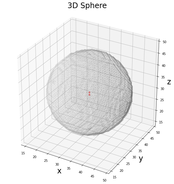
As expected, for a 3D sphere the number of points belonging to the skeleton is not sufficient for the identification of a network, since the skeleton is given by the center of the sphere. The application of the filter is useless in this case.

NOTE: Despite the mathematical solution of the skeleton for the 3D sphere should provide only the center of the sphere, i.e. 1 point, the Lee skeletonization returns a couple of points! This behaviour is due to the structural element used for the definition of the sphere. Considering a sphere of radius 1 we can describe it as a cross element, a single voxel or a 2x2x2 cube. All these definitions are correct and lead to different definition of the center of the sphere as belonging to a “real” voxel or to an “half” voxel. According to the different definitions we can obtained different results as skeleton.

Cylinder

def cylinder (shape: tuple, height: int, radius: int, position: tuple):
    '''
    Generate an n-dimensional cylindral mask.
    '''
    arr = np.zeros(shape, dtype=bool)
    x, y, z = shape
    x0, y0 = position

    # xx and yy are XY tables containing the x and y coordinates as values
    # mgrid is a mesh creation helper
    xx, yy = np.mgrid[:x, :y]
    # circles contains the squared distance to the central point
    # we are just using the circle equation learnt at school
    circle = (xx - x0) ** 2 + (yy - y0) ** 2

    circle = circle < radius**2
    start = z//2 - height//2
    stop  = start + height # i.e z//2 + height//2

    for i in range(start, stop):
        arr[..., i] = circle

    return arr

# create a 3D cylinder as volume mask
volume = cylinder(shape=(64, 64, 64), height=32, radius=8, position=(32, 32))
sitk_volume = sitk.GetImageFromArray(np.uint8(volume))

# get the 3D skeleton of the object
skeletonizer.Execute(sitk_volume)
skeleton = skeletonizer.GetSkeletonImage()

# execute the filter
extractor.Execute(skeleton)

# get the returning values
nodes = extractor.GetNodeIndexes()
edges = extractor.GetEdgeIndexes()
edgeLUT = extractor.GetEdgeLUTIndexes()
edges_lbl = extractor.GetEdgeMap()

# extract the 3D mesh of the object for the plot
verts, faces, normals, values = marching_cubes(volume, 0)

# plot the results
fig = plt.figure(figsize=(10, 10))
ax = fig.add_subplot(projection='3d')

# draw the skeleton shape
sz, sy, sx = np.where(sitk.GetArrayViewFromImage(skeleton))
if len(sx):
    ax.scatter(sx, sy, sz, color='r', marker='o', s=20, alpha=0.5)
else:
    print('No skeleton found')

# plot the nodes as blue dots
if len(nodes):
    ax.scatter(*zip(*nodes), color='b', marker='o', s=50)
else:
    print('No nodes found in the Graph')

# plot the edges as lines between vertices
for ex, ey in edges:
    ax.plot(*zip(*(ex, ey)), color='lime', linewidth=2)

# draw the object volume
ptz, pty, ptx = verts.T
ax.plot_trisurf(ptx, pty, faces, ptz,
                color='lightgray',
                alpha=0.1,
                antialiased=False,
                linewidth=0.0
               )
ax.set_box_aspect((np.ptp(ptx), np.ptp(pty), np.ptp(ptz)))
ax.set_xlabel('x', fontsize=24)
ax.set_ylabel('y', fontsize=24)
ax.set_zlabel('z', fontsize=24)
_ = ax.set_title('3D Cylinder', fontsize=24)

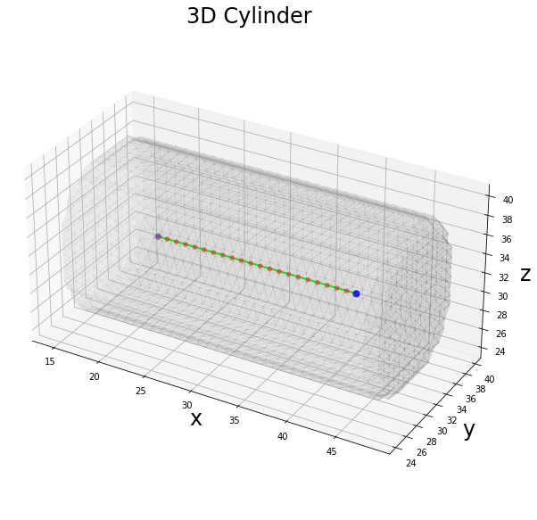
The skeleton of a 3D cylinder is given by the central axis along the major dimension of the volume. Since the skeleton is given by just a segment, the corresponding graph will have 2 nodes (the extreme points of the segment) and 1 link (the segment which connect the two extremes). In this case the corresponding graph can be modeled as a chain.

Cube

def cube (shape: tuple, side: int):
    '''
    Generate an n-dimensional cube mask.
    '''
    arr = np.zeros(shape, dtype=bool)
    x, y, z = shape

    start = z//2 - side//2
    stop  = start + side # i.e z//2 + side//2

    arr[start:stop, start:stop, start:stop] = True

    return arr

# create a 3D cube as volume mask
volume = cube(shape=(64, 64, 64), side=32)
sitk_volume = sitk.GetImageFromArray(np.uint8(volume))

# get the 3D skeleton of the object
skeletonizer.Execute(sitk_volume)
skeleton = skeletonizer.GetSkeletonImage()

# execute the filter
extractor.Execute(skeleton)

# get the returning values
nodes = extractor.GetNodeIndexes()
edges = extractor.GetEdgeIndexes()
edgeLUT = extractor.GetEdgeLUTIndexes()
edges_lbl = extractor.GetEdgeMap()

# extract the 3D mesh of the object for the plot
verts, faces, normals, values = marching_cubes(volume, 0)

# plot the results
fig = plt.figure(figsize=(10, 10))
ax = fig.add_subplot(projection='3d')

# draw the skeleton shape
sz, sy, sx = np.where(sitk.GetArrayViewFromImage(skeleton))
if len(sx):
    ax.scatter(sx, sy, sz, color='r')
else:
    print('No skeleton found')

# plot the nodes as blue dots
if len(nodes):
    ax.scatter(*zip(*nodes), color='b', marker='o', s=50)
else:
    print('No nodes found in the Graph')

# plot the edges as lines between vertices
for ex, ey in edges:
    ax.plot(*zip(*(ex, ey)), color='lime', linewidth=2)

# draw the object volume
ptz, pty, ptx = verts.T
ax.plot_trisurf(ptx, pty, faces, ptz,
                color='lightgray',
                alpha=0.1,
                antialiased=False,
                linewidth=0.0
               )
ax.set_box_aspect((np.ptp(ptx), np.ptp(pty), np.ptp(ptz)))
ax.set_xlabel('x', fontsize=24)
ax.set_ylabel('y', fontsize=24)
ax.set_zlabel('z', fontsize=24)
_ = ax.set_title('3D Cube', fontsize=24)

No skeleton found
No nodes found in the Graph

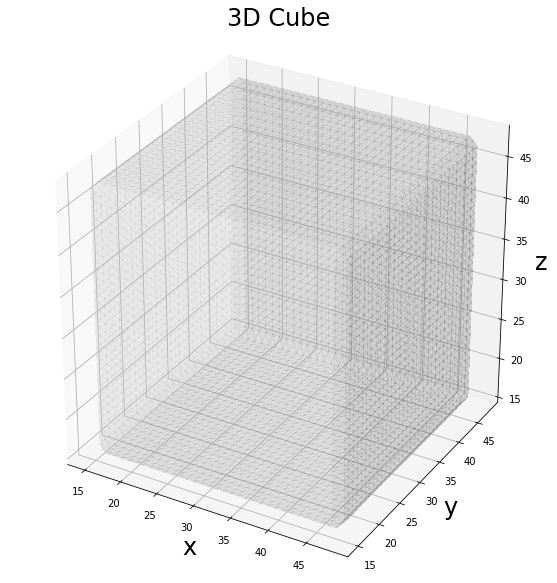
As for the case of the sphere, neither the 3D cube has a skeleton backbone according to the definition of the Lee algorithm. Therefore, we cannot define any internal graph.

Hollow Sphere

# create a 3D hollow sphere as volume mask
external = sphere(shape=(64, 64, 64), radius=16, position=(32, 32, 32))
hollow = sphere(shape=(64, 64, 64), radius=8, position=(32, 32, 32))
volume = external ^ hollow
sitk_volume = sitk.GetImageFromArray(np.uint8(volume))

# get the 3D skeleton of the object
skeletonizer.Execute(sitk_volume)
skeleton = skeletonizer.GetSkeletonImage()

# execute the filter
extractor.Execute(skeleton)

# get the returning values
nodes = extractor.GetNodeIndexes()
edges = extractor.GetEdgeIndexes()
edgeLUT = extractor.GetEdgeLUTIndexes()
edges_lbl = extractor.GetEdgeMap()

# extract the 3D mesh of the object for the plot
verts, faces, normals, values = marching_cubes(volume, 0)

# plot the results
fig = plt.figure(figsize=(10, 10))
ax = fig.add_subplot(projection='3d')

# draw the skeleton shape
sz, sy, sx = np.where(sitk.GetArrayViewFromImage(skeleton))
if len(sx):
    ax.scatter(sx, sy, sz, color='r', marker='o', s=20, alpha=0.5)
else:
    print('No skeleton found')

if len(nodes):
    # plot the nodes as blue dots
    ax.scatter(*zip(*nodes), color='b', marker='o', s=50)
else:
    print('No nodes found in the Graph')

# plot the edges as lines between vertices
for ex, ey in edges:
    ax.plot(*zip(*(ex, ey)), color='lime', linewidth=2)

# draw the object volume
ptz, pty, ptx = verts.T
ax.plot_trisurf(ptx, pty, faces, ptz,
                color='lightgray',
                alpha=0.1,
                antialiased=False,
                linewidth=0.0
               )
ax.set_box_aspect((np.ptp(ptx), np.ptp(pty), np.ptp(ptz)))
ax.set_xlabel('x', fontsize=24)
ax.set_ylabel('y', fontsize=24)
ax.set_zlabel('z', fontsize=24)
_ = ax.set_title('3D Sphere', fontsize=24)

No nodes found in the Graph

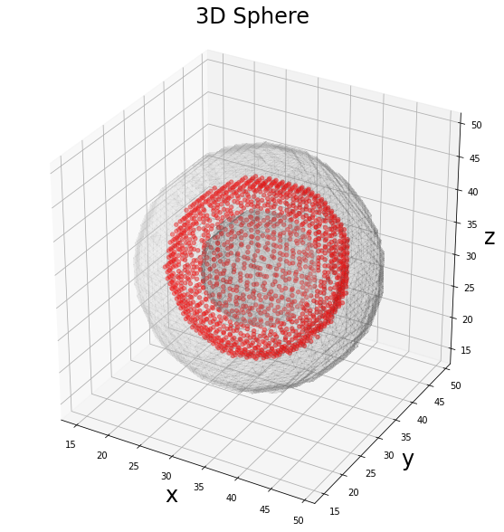
The case of the Hollow Sphere is a “particular” case, since the definition of the skeleton in relation to concavities is not trivial. We commonly think about the skeleton as a line/axis while in 3D geometry its definition could be extended also to surfaces. This is the case of the hollow sphere, in which the concavity leads to a skeleton given by a sphere itself. In this case we cannot define a graph, expecially because we have built our graph-extractor setting the remove_surface parameter as True.

Analogous results can be obtained considering an Hollow Cylinder or an Hollow Cube. For sake of brevity we have analyzed only the Hollow Sphere as case study.

Random Blob

from skimage.data import binary_blobs

# Generate 3D random blobs
volume = binary_blobs(length=64,
                      blob_size_fraction=.5,
                      volume_fraction=.1,
                      seed=42,
                      n_dim=3
                     )
sitk_volume = sitk.GetImageFromArray(np.uint8(volume))

# get the 3D skeleton of the object
skeletonizer.Execute(sitk_volume)
skeleton = skeletonizer.GetSkeletonImage()

# execute the filter
extractor.Execute(skeleton)

# get the returning values
nodes = extractor.GetNodeIndexes()
edges = extractor.GetEdgeIndexes()
edgeLUT = extractor.GetEdgeLUTIndexes()
edges_lbl = extractor.GetEdgeMap()

# extract the 3D mesh of the object for the plot
verts, faces, normals, values = marching_cubes(volume, 0)

# plot the results
fig = plt.figure(figsize=(10, 10))
ax = fig.add_subplot(projection='3d')

# draw the skeleton shape
sz, sy, sx = np.where(sitk.GetArrayViewFromImage(skeleton))
ax.scatter(sx, sy, sz, color='r', marker='o', s=20, alpha=0.5)

# plot the nodes as blue dots
ax.scatter(*zip(*nodes), color='b', marker='o', s=50)

# plot the edges as lines between vertices
for ex, ey in edges:
    ax.plot(*zip(*(ex, ey)), color='lime', linewidth=2)

# draw the object volume
ptz, pty, ptx = verts.T
ax.plot_trisurf(ptx, pty, faces, ptz,
                color='lightgray',
                alpha=0.05,
                antialiased=False,
                linewidth=0.0
               )
ax.set_box_aspect((np.ptp(ptx), np.ptp(pty), np.ptp(ptz)))
ax.set_xlabel('x', fontsize=24)
ax.set_ylabel('y', fontsize=24)
ax.set_zlabel('z', fontsize=24)
_ = ax.set_title('3D Blobs', fontsize=24)

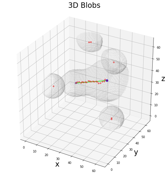
This is the most general case, in which random 3D shapes can occur. In this case the graph extractor will return a subgraph for each connected component found in the 3D volume, according to a 8-connectivity. Since not all the 3D shapes allow the definition of a graph (in this case), the number of the graph connected components is reduced to the only available ones.